Predictive Analytics with Machine Learning and Databricks Series Pt 2

“Starting Up a Cluster”

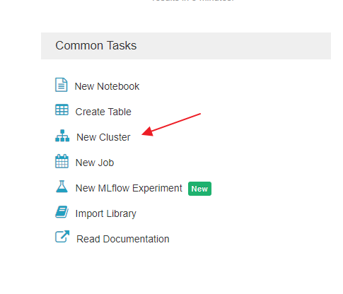
In the first part of this four-part series we focused on getting comfortable with the console. In this blog and second part of our series we will focus on starting up your first cluster. In Databricks the interactive GUI guides step by step in standing up the cluster. Under common tasks click on “New Cluster”.

Once you start creating a new cluster you will be prompted with the following screen:

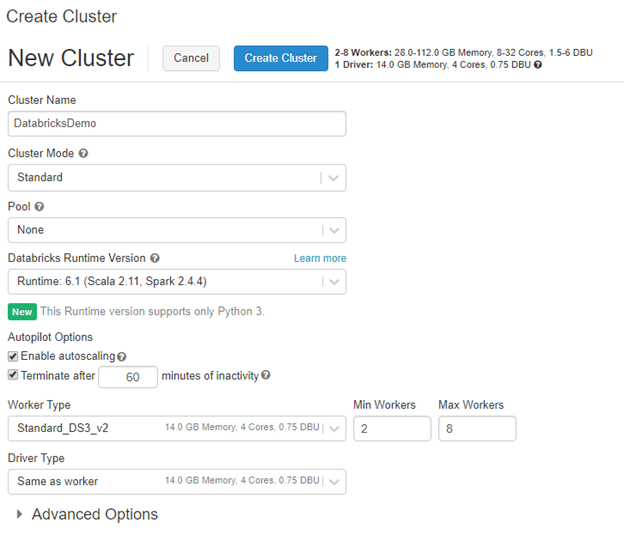
Let’s discuss some of these options so that you have a general understanding of what you’re doing. The cluster name is what your naming your cluster. Cluster mode has two options:

• High Concurrency
• Standard

By default, Databricks will use standard. The difference between the two is high concurrency is optimized to run Python, R, and SQL. It’s important to note that high concurrency does not support Scala. Whereas with standard you are leveraging a single-user cluster and can run Python, R, Scala, and SQL.

Pools are used to have standby clusters up and ready. The use case for this is when you have a heavy workload that requires a larger amount of nodes you can optimize for that workload but can turn them off to save money. What about the time it takes to stand a cluster back up? How many nodes are in the cluster? Well pools allow for you to utilize those standby clusters to reduce the wait for clusters to be ready for the next job without having all resource online all of the time.

Runtime versions vary based on need. I would highly suggest doing some reading on them. At the time of writing this blog the default is Runtime 6.1 (Scala 2.11 and Spark 2.4.4). Runtime versions all about scalability and performance. There is also an option here for Machine Learning which is geared towards optimizing machine learning productivity.

Worker types and driver types are similar to sizing a VM for the workload that it will be handling. These identify the memory, cores, and DBU that will be associated the given cluster you are building.

With that being said I am going to select Runtime 6.1 ML. I am choosing this version because later in this series we will also use SQL which is not supported in 6.1 without the ML option.

Once selected it will take a few minutes for the cluster to stand up. But you will be redirected to a screen that should show your cluster is in a pending status. Give it a few seconds for the cluster to show in the interactive cluster window.

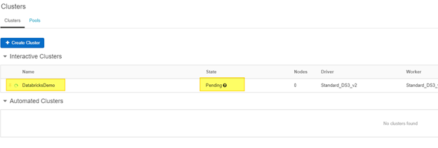
Now I know you are wondering the difference between an interactive cluster and an automated cluster. So to make it short and sweet. An interactive cluster lets up collaboratively analyze data with interactive notebooks. While an automated cluster is setup for automating jobs to train data as it comes into your model. Here is quick link from Microsoft that dives a little further into the differences between the two cluster types.

If you’re still following along, I hope your looking forward to the next part(s) of this series that will go over training your model and scoring your results. Once we get there we will then look at ways to visually represent you model scores and data. Stay tuned for part 3!